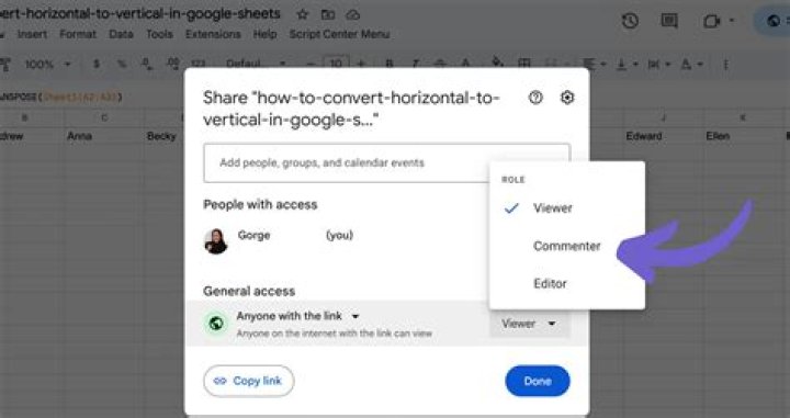
How to Hide Formulas in Google Sheets Using Protected Sheets and Ranges

1. Select the range of cells containing the formulas you want to hide.
2. Select Protected sheets and ranges under the Data menu.
3. In the pop-up window, select Set Permissions.
4. In the dialog box, choose Restrict who can edit this range.

Why formula is not working in Google Sheets?

One of the first things you want to try when your formulas aren’t working properly is a simple refresh on your spreadsheet. To do this in the top left corner of your browser select the refresh button. You can also press F5 on your keyboard to refresh. Sometimes a simple refresh will fix your problems.

How do you stop Excel from thinking it’s a formula?

How do I stop Excel from automatically changing the format of my formula to text?

1. Press Ctrl+H.
2. In the find what box, type =
3. In the Replace with box, type = (again)
4. Click on Replace All.

How do I create a formula for an entire column in Google Sheets?

Drag the cell’s handle to the bottom of your data in the column. Click the small blue square at the bottom-right of the cell and drag it down across all the cells you want to apply the formula to. When you release the click, the formula from the first cell will be copied into every cell in your selection.

What does F4 do in Google Sheets?

Press the F4 key to toggle between relative and absolute references in ranges in your Google Sheets formulas. It’s WAY quicker than clicking and typing in the dollar ($) signs to change a reference into an absolute reference.

Why is match function not working?

If you believe that the data is present in the spreadsheet, but MATCH is unable to locate it, it may be because: The cell has unexpected characters or hidden spaces. The cell may not be formatted as a correct data type. For example, the cell has numerical values, but it may be formatted as Text.

Why isn’t my Importrange working?

There are many approaches to fixing this issue: Hard refresh of the sheet and/or browser. Re-adding the IMPORTRANGE formula to the same cell (use the Google Sheets shortcuts Ctrl+X and then Ctrl+V or clear the cell and use Ctrl+Z to restore it) Nest IMPORTRANGE with IFERROR.

Why does Excel think is a formula?

The next reason why formulas are shown as formulas: You may have set the cell formatting to “Text” and then typed the formula in it. When you set the cell formatting to “Text”, Excel treats the formula as text and shows it instead of evaluating it. Now edit the formula and press enter.

Why is Excel changing my formula?

Usually the CELL REFERENCES will CHANGE! If you copy a formula 3 rows down and 1 row left, then the cell references in the formula will shift 3 rows down and 1 row left. These are called “relative” cell references, since they change relative to where you copy the formula.

How do I copy a formula down an entire column?

You can always use the good ole’ copy and paste method.

1. Set up your formula in the top cell.
2. Either press Control + C or click the “Copy” button on the “Home” ribbon.
3. Select all the cells to which you wish to copy the formula.
4. Either press Control + V or click the “Paste” button on the “Home” ribbon.

How do I apply a formula to an entire column in Google sheets without dragging?

Then press Ctrl+Shift+Enter, or Cmd+Shift+Enter on Mac, and Google Sheets will automatically surround your formula with ARRAYFORMULA function. Thus, we could apply the formula to the entire column of the spreadsheet with only a single cell.

How do you use F4 in sheets?

How do you F4 in Google Sheets?

Keyboard Shortcut – F4 When typing your formula, immediately after clicking on a cell to select it for your formula select the F4 key. Striking the F4 key once will create double dollar signs on that cell reference.

How does match formula work?

The MATCH function searches for a specified item in a range of cells, and then returns the relative position of that item in the range. For example, if the range A1:A3 contains the values 5, 25, and 38, then the formula =MATCH(25,A1:A3,0) returns the number 2, because 25 is the second item in the range.

What does match return if no match?

When the function cannot find an exact match, it will return the position of the closest match above the lookup_value. (If this option is used, the lookup_array must be in descending order).

How do I enable Importrange?

About Granting Access With IMPORTRANGE

1. Spreadsheets must be explicitly granted permission to pull data from other spreadsheets using IMPORTRANGE.
2. The first time the destination sheet pulls data from a new source sheet, the user will be prompted to grant permission.

How do you refresh Importrange?

1. Open you Spreadsheet and click File -> “Spreadsheet” settings.
2. In “Recalculation” section, choose your best setting from the drop-down menu: On change / On change and every minute / On change and every hour.
3. Click “Save Settings”.

What’s wrong with this formula in Excel?

Excel formula error is generated when one of the variables in a formula is of the wrong type. For example, the simple formula =B1+C1 relies on cells B1 and C1 containing numeric values. Therefore, if either B1 or C1 contains a text value, this results in the #VALUE!

How do I create a formula in Google Sheets?

Use a formula

1. Open a spreadsheet.
2. Type an equal sign (=) in a cell and type in the function you want to use.
3. A function help box will be visible throughout the editing process to provide you with a definition of the function and its syntax, as well as an example for reference.

How do you calculate on a spreadsheet?

To do this you select a cell in a new column or row and then type in a formula. A formula starts with an equals sign (=) that tells the spreadsheet you want to do a calculation. A formula then has a symbol for what kind of calculation you want to perform (add, subtract, multiply, divide, etc.).

How to create simple formulas in Google Sheets?

By combining a mathematical operator with cell references, you can create a variety of simple formulas in Google Sheets. Formulas can also include a combination of a cell reference and a number.

How can Google Sheets be used for calculations?

When working with numerical information, Google Sheets can be used to perform calculations. In this lesson, you’ll learn how to create simple formulas that will add, subtract, multiply, and divide values. You will also be introduced to the basics of using cell references in formulas.

How do you make a Google challenge sheet?

Make sure you’re signed in to Google, then click File > Make a copy. Select the Challenge sheet. In cell D4, create a formula that multiplies cells B4 and C4. Be sure to use cell references. Use the fill handle to copy the formula to cells D5 and D6.

What is the formula for split in Google Sheets?

All you have to do is type the following formula: =SPLIT (B3,“ ”) into Cell C3, and you’ll see your prospect’s first and last names appear in cells C3 and D3. Then drag Cell C3 downwards to populate the rest of the cells. That’s all there is to it!